r1.32과 현재 버전의 차이점
@@ -1,1049 +1,199 @@
% autosam.tex
% Annotated sample file for the preparation of LaTeX files
% for the final versions of papers submitted to or accepted for
% publication in AUTOMATICA.
% See also the Information for Authors.
% Make sure that the zip file that you send contains all the
% files, including the files for the figures and the bib file.
% Output produced with the elsart style file does not imitate the
% AUTOMATICA style. The style file is generic for all Elsevier
% journals and the output is laid out for easy copy editing. The
% final document is produced from the source file in the
% AUTOMATICA style at Elsevier.
% You may use the style file autart.cls to obtain a two-column
% document (see below) that more or less imitates the printed
% Automatica style. This may helpful to improve the formatting
% of the equations, tables and figures, and also serves to check
% whether the paper satisfies the length requirements.
% Please note: Authors must not create their own macros.
% For further information regarding the preparation of LaTeX files
% for Elsevier, please refer to the "Full Instructions to Authors"
{{|
% from Elsevier'
s anonymous ftp server on ftp.elsevier.nl in the
% directory pub/styles, or from the internet (CTAN sites) on
''이 페이지는 마음껏 [테스트]를 위한 곳입니다'''
% ftp
약간의 설명이 있는 연습장 원하시는 분은 WikiSandBox로 가시기 바랍니다.
shsu.edu, ftp.dante.de and ftp.tex.ac.uk in the directory
% tex-archive/macros/latex/contrib/supported/elsevier.
%\documentclass{elsart
|}
% The use of LaTeX2e is preferred.
\documentclass{autart}
% The use of LaTeX2e is preferred.
%\documentclass[twocolumn]{autart} % Enable this line and disable the
% preceding line to obtain a two-column
% document whose style resembles the
% printed Automatica style.
[[HTML(<center>*******</center>)]]
$$\cos x$$
\usepackage{graphicx} % Include this line if your
% document contains figures,
%\usepackage[dvips]{epsfig} % or this line, depending on which
% you prefer.
\usepackage{amsmath}
\usepackage{cuted,flushend}
== 테스트를 해보자 ==
$$\int_{\infty}^{\infty}\oint\mathop{\lim}\limits_{a \to \infty}(가)$$
\def\nr{\nonumber \\}
sd
\begin{document}
fsadf
asdf
sadf
ㅎ나글은 머냐? 거시기? 어쩌라공 ㅋㅋ
ㅇㅇㅇ
$$\
begin
int_{
frontmatter
\infty}
%
^{\
runtitle
infty}\oint\mathop{\lim}\limits_{
Insert a
suggested running title
\to \infty}
% Running title for regular
% papers but only if the title
% is over 5 words. Running title
% is not shown in output.
(가)$$
$$\
title
sqrt{
Risk Sensitive FIR Filters for Stochastic
ab}$$
Discrete-time State Space Models\thanksref{footnoteinfo}} % Title, preferably not more
== 연습장 ==
% than 10 words.
Wave equation is
\thanks[footnoteinfo]{This paper was not presented at any IFAC
meeting and was supported by the Post-doctoral Fellowship Program
of Korea Science \& Engineering Foundation(KOSEF). Corresponding
author Wook Hyun Kwon. Tel. +82-2-880-7307. Fax +82-2-871-7010. }
112112
$$ \
author[Rome]
mbox{
sungho Jang
한글}
\ead
$$
$x^2$
B)
123tyt굣ㅛㅅㅅㄱㄳ견ㅇ탸ㅏfdsarㅏgbvfdwgregregqㅓㅊ허ㅠㅊv+987{
shjang@icat.snu.ac.kr
il}
, % Add the
32
$$ \
author[Rome]
mbox{
Wook Hyun Kwon
한글}
\ead{whkwon@cisl
$$
$x^2$
B)
== 번호달린 목록 ==
1.
snu
aaa
1.
ac
bbb
1.
kr} % e-mail address
ccc
% (ead
1. dddfd:)
as shown
1. eee
1. fff
2. fdmskmsdaokgnqokfsdamnkl
== Google Equation Editor를 이용한 수식 입력 연습 ==
[[HTML(<script src="http://gmodules.com/ig/ifr?url=http://www.sitmo.com/gg/latex/latex.xml&up_eq=&up_z=100&synd=open&w=320&h=500&title=Equation+Editor&border=%23ffffff%7C3px%2C1px+solid+%23999999&output=js"></script>)]]
\address[Rome]{ Engr. Research Center for Advanced Contr. and Instru.,and\\
School of Electrical Engr. $\&$ Computer Science, Seoul Nat'l Univ., Seoul,
151-742, Korea.} % full addresses
== MetaPost Processor ==
{{{#!metapost
pickup pencircle scaled 1pt;
path px,py,ps;
t=180/3.1416; u=1cm;
\begin{keyword} % Five to ten keywords,
Risk sensitive; Risk averse; Risk seeking
ps=(-2.
% chosen from the IFAC
\end{keyword} % keyword list or with the
% help of the Automatica
% keyword wizard
\begin{abstract} % Abstract of not more than 200 words.
In this paper
5,
the finite impulse response
sind(
FIR
-2.5t))
filter based on an
*u
exponential quadratic cost function is proposed for
a stochastic
discrete
i=-
time state space model
2.
The joint probability density
function for variables on the recent finite horizon is introduced
and the corresponding expected value of the exponential quadratic
cost function is minimized
4 step 0.
According to the sign of the scalar
real parameter in the cost function, we obtain a risk averse or
seeking FIR filter, called a risk sensitive FIR filter
1 until 2.
Being risk
averse means that large weights are put on large estimation
errors
5: --(i,
which are suppressed as much as possible. Being risk
seeking means that large weights are put on moderate estimation
errors. It is shown that the risk averse or seeking FIR filter
reduces to a minimum variance FIR filter that is more general than
existing ones. It is also shown via simulation that the proposed
FIR filter has the better performance than the conventional
infinite impulse response
sind(
IIR
i*t)
Kalman filter.
\end{abstract}
\end{frontmatter}
%%%%%%%%%%%%%%%%%%%%%%%%%%%%%%%%%%%%%%%%%%%%%%%%%%%%%%%%%%%%%%%%%%%%
%%%%%%%%%%%%%%%%%%%%%%%%%%%%%%%%%%%%%%%%%%%%%%%%%%%%%%%%%%%%%%%%%%%%
%%%%%%%%%%%%%%%%%%%%%%%%%%%%%%%%%%%%%%%%%%%%%%%%%%%%%%%%%%%%%%%%%%%%
\section{Introduction}
%%%%%%%%%%%%%%%%%%%%%%%%%%%%%%%%%%%%%%%%%%%%%%%%%%%%%%%%%%%%%%%%%%%%
%%%%%%%%%%%%%%%%%%%%%%%%%%%%%%%%%%%%%%%%%%%%%%%%%%%%%%%%%%%%%%%%%%%%
%%%%%%%%%%%%%%%%%%%%%%%%%%%%%%%%%%%%%%%%%%%%%%%%%%%%%%%%%%%%%%%%%%%%
The estimation of the unknown values from given measurements
arises in many fields such as control, signal processing, and
communications. Specially, how to estimate a state from
measurements on a state space model has been extensively exploited
since most dynamic systems can be easily described over state
spaces.
)*u endfor;
For a long time, the optimal estimators or filters for state
estimations have been developed on the basis of the
Luenberger
px=(-
type filters such as the
Kalman filter\cite{Kalman60} and the $H_{\infty}$ filter\cite{Nagpal91}. %The Kalman
%filter\cite{Kalman60} is designed so that the variance of the
%estimation error is minimized. In case that the stochastic
%information is not available and the worst case should be
%considered
4u,
the $H_{\infty}$ filter \cite{Nagpal91} has been
%devised. Starting from two representative filters, many variants
%have been proposed for I/O models \cite{has:ind99}, robustness
%\cite{Xie94}, fast computation \cite{Sayed94}, and so on.
The duration of impulse response of the conventional Kalman and
$H_{\infty}$ filters is infinite, which means that these filters
belong to infinite impulse response(IIR
0)
filters in a signal
processing area. Actually, these days
--(4u,
these IIR filters give ways
to finite impulse response
0); py=(
FIR
0,-2u)
filters in the signal processing
area. It is generally known that the FIR filters are robust
against temporary modelling uncertainties or round-
off errors. FIR
filters can resolve the divergence and the slow convergence known
as demerits of IIR filters.
-(0,2u);
While IIR filters for state estimations have been widely used for
a long time, FIR filters for that purpose have not received much
attention and have not been researched much. As in the signal
processing area, undesirable effects of the IIR filters for state
estimations may be alleviated by using the FIR structure. In this
paper, we consider an FIR filter given by
\begin{eqnarray}
\hat{x}_{k}&=& \sum_{i = k-N}^{{k-1}} H_{k-i} y_{i} + \sum_{i =
k-N}^{{k-1}} L_{k-i}u_{i}, \label{firfilter}
\end{eqnarray}
for some gains $H_\cdot$ and $L_\cdot$. The basic block diagram of
the FIR filter
fill buildcycle(
\ref{firfilter}) is depicted in Fig.
\ref{fig:fir_filter}.
\begin{figure}
\begin{center}
\includegraphics[scale=0.5]{fir_filter.eps}
\end{center}
\caption{Block diagram of FIR filter : D is a unit delay
component} \label{fig:fir_filter}
\end{figure}
By using a forgetting factor
ps,
there have been trials mimicking
(\ref{firfilter})\cite{Yang97}
px,
which may be called a soft FIR
filter if the FIR filter
py shifted (
\ref{firfilter}) is called a hard FIR
filter. Besides
2u,
the Kalman filter is forced to put more weights
on the recent data like the FIR filter (\ref{firfilter}
0)
, if
necessary, by increasing a system noise
covariance\cite{bur:lin98}. However, these methods are very
heuristic and spoil the optimality for the given performance
criteria. In this paper, filter coefficients $H_{\cdot}$ and
$L_{\cdot}$ in (\ref{firfilter})
will be computed to optimize the
given performance criterion. Among linear FIR filters of the form
withcolor blue;
fill buildcycle(
\ref{firfilter})
ps,
we will obtain the filter for the following
performance criterion:
\begin{eqnarray}
\min_{\hat x_k} ~ -\frac{2}{\alpha} \log \big [ \textbf{E} e^{
-\frac{\alpha}{2} e_k^T e_k } \big]
px,
\label{ch4:mvf:cost_rel}
\end{eqnarray}
where $\alpha$ is a constant, $\mathbf{E}
py shifted (
\cdot)$ denotes the
expectation, and $ e_k \stackrel{\triangle}{=} \hat x_{k} -
x_k$
is the estimation error at the time $k$. $-\frac{2}{\alpha} \log$
in
(\ref{ch4:mvf:cost_rel}) is just a scaling factor. %For $\alpha<0$
%and $\alpha>0$
2u,
The criterion (\ref{ch4:mvf:cost_rel}) is equivalent to minimizing
$\mathbf{E}[-\frac{2}{\alpha}(e^{-\frac{\alpha}{2}e^T_k e_k }-1)]$
since a logarithmic function is monotonic increasing and a
constant term is not involved with the operation of an
expectation. How $-\frac{2}{\alpha} (e^{-\frac{\alpha}{2}e^T_k e_k
}-1)$ varies with $e_k^T e_k$ for different values of $\alpha$ is
shown in Fig. \ref{fig:cost_function}. Sharpness and dullness of
the graph can be varied with the value of $\alpha$. As $\alpha$
goes to zero, $-\frac{2}{\alpha} (e^{-\frac{\alpha}{2}e^T_k e_k
}-1)$ reduces to $e^T_k e_k$ so that the criterion
(\ref{ch4:mvf:cost_rel}) is equivalent to the minimum variance
one. It can be said that the criterion (\ref{ch4:mvf:cost_rel}) is
a general version of the minimum variance one. For $\alpha<0
$, the
cost function (\ref{ch4:mvf:cost_rel})
is called a risk averse
criterion since large weights are put on large estimation errors
and thus the large or risky estimation errors would be suppressed
as much as possible. This also means that the designer is
pessimistic about the estimation errors so that the filter based
on this criterion will work well when large estimation errors
often happen. For $\alpha>0$, the cost function
(\ref{ch4:mvf:cost_rel})
is called a risk seeking criterion since
large weights are put on moderate estimation errors and large
estimation errors are less weighted compared with the risk averse
criterion for $\alpha<
withcolor red;
0$.
%, which comes from the fact that the cost function
%(\ref{ch4:mvf:cost_rel_1}) becomes the minimum for the moderate
%$\textbf{E}[e_k e_k^T]$. How moderate a given noise is depends on
%$\alpha$.
It is useful when the occasional occurrence of a large estimation
error is tolerable. This also means that the designer is
optimistic about the estimation errors so that the filter based on
this criterion will work well when estimation errors are mostly
moderate. The FIR filter based on risk averse or seeking criteria
is called a risk sensitive FIR filter(RSFF).
\begin{figure}
\begin{center}
\includegraphics[scale=0.4]{cost.ps}
\end{center}
\caption{ Cost functions vs $e_k^T e_k$ }
\label{fig:cost_function}.
\end{figure}
There have been a few results on FIR filtering for limited models
and heuristic approaches. For deterministic discrete
drawarrow px; % X-
time systems
without noises, a moving horizon least-square filter of the form
(\ref{firfilter}) was given in \cite{Ling99}. For special discrete
stochastic systems without system noises, a linear FIR filter was
introduced from a maximum likelihood criterion \cite{Jazw68}.
Since the system noise is not considered, the FIR filter is of the
simple form and easy to derive. For general discrete-time
stochastic systems, FIR filters were introduced by a modification
from the Kalman filter \cite{RDKwon99} where the infinite
covariance of the initial state information is difficult to handle
and the efficiency of the filters is not clear. Besides, this work
brings out a limitation that the system matrix is required to be nonsingular. %In the above
%papers, unbiasedness was checked after the optimal filters were
%obtained. In this paper, unbiased condition will be built in
%during design procedure. %If it is assumed that the system matrix
%is nonsingular or the system noise is removed, the derivation of
%the FIR filter
axis
drawarrow py; %
for discrete
Y-
time systems becomes somewhat easy. %That is why many
axis
draw ps; %
previous results were based on these assumptions.
Sine curve
In \cite{whkwon00}
, the optimal FIR filter with the unbiased
condition was given under an assumption that the system matrix is
nonsingular. Even though the unbiased condition leads to an easy
derivation, it may go against the optimality of the performance
criterion. In \cite{Ling99}
, the FIR filter was derived without
this assumption. Instead, the system noise was assumed not to
exist.
}
To the authors' knowledge, there is no result about FIR filters
for general state space models without any artificial restrictions
or conditions which may prevent FIR filters from applying to
real applications. %For example, in case of high order systems, the
%system matrix may be a sparse matrix so that there is a high
%probability that the system matrix is singular.
Practically, some system matrices may be singular. Even though the
matrix is nonsingular, the inverse operation may cause critical
numerical errors. If filters are designed without consideration of
noises, these may not have the good performance in case that
noises appear. In this paper, we will derive FIR filters without
these constraints for the criterion (\ref{
ch4:mvf:cost_rel}) which
{{#!latex
includes a minimum variance criterion with $\alpha
=0$
as mentioned
before. General systems with the system and measurement noises
will be considered and the inverse of the system matrix is not
required, \emph{i.e.}
, $H_{\cdot}
$ and $L_{\cdot}
$ of
(\ref{firfilter}) will be represented without using the inverse of
the system matrix. The unbiased condition for easy derivation will
not be employed during the design. While the existing results are
based on the minimum variance or least square criteria, this paper
deals with the more general performance criteria
(\ref{ch4:mvf:cost_rel}). It is shown that the FIR filter based on
the criterion (\ref{ch4:mvf:cost_rel}) is independent of the value
$\alpha$. It means that the proposed RSFF is also optimal in view
of a minimum variance criterion of the case $\alpha=0$. To put it
other way, the RSFF can be a generalized version of existing
minimum variance FIR filters since any artificial restrictions or
conditions are not taken.
%If $\alpha$ goes to zero, the proposed RSFF reduces to the minimum
%variance FIR filters.
%Thus it is desirable to derive FIR filters without these
%constraints.
%In this paper, a discrete-time FIR filter with {\it{a priori}}
%built-in unbiasedness condition will be given without a
%requirement of a system matrix.
%To the authors' knowledge, there is no result about FIR filters
%that are derived for general state space models without any
%restriction such as the existence of the inverse of the system
%matrix. In this paper, the new FIR filters are proposed for the
%general systems with the system and measurement noises, and do not
%require the inverse of the system matrix, \emph{i.e.}, $H_{\cdot}$
%and $L_{\cdot}$ of (\ref{firfilter}) will be represented without
%using the inverse of the system matrix. Additionally, in this
%paper, the more general performance criteria
%are employed instead of the minimum variance criterion. %Actually,
%it is shown that the RAFF is not dependent on $\alpha$ in
%(\ref{ch4:mvf:cost_rel}), which means that the RAFF is also
%optimal for minimum variance criterion. It is a surprising fact
%that the minimum variance FIR filter has the risk averse property.
%The proposed RAFF is different from the existing minimum variance
%FIR filer in that the first is based on general stochastic systems
%and does not require the nonsingularity of the system matrix. The
%proposed RSFF is obtained in a numerical way while the RAFF is
%obtained in a closed form.
WikiWiki한글
For a long time, robustness has been addressed for the analysis
----
and the design of the IIR filters for state estimations. It was
:)
shown in
== 군(群 ; group)의 정의 ==
\cite{Heffes66}\cite{Price68}\cite{Fitz71}\cite{Toda80}\cite{Iam90}
KTUGBoard:2641
that the conventional IIR filter,
연산 $\
emph{i.e.}
times$ 가 정의된 공집합이 아닌 집합 $G$ 가 다음 4가지 조건을 만족하면,
the Kalman filter
can diverge and has the poor performance due to model
uncertainties. In order to build up robustness, robust Kalman and
$
H_{\infty}
G$
filters were proposed in \cite{Xie94}\cite{Souza94}.
In several works\cite{Ang:rec03,Ang:Est04,MHE:Rao99}, it was shown
through simulation and a quantitative analysis that the FIR
filtering for state estimations could also be a good substitute to
achieve a high
degree of robustness as in the signal processing area. %It is
%really worth making comparisons of a robustness improvement due to
%the FIR structure and the robust design of IIR filters.
Through simulation, we will show that the proposed RSFF has the
robustness to model uncertainties
를 군(群)이라 한다.
In Section 2 and 3, the RSFF is derived
* [단위원] $e(가)$ 가 존재한다.
In Section 4, it is shown
via simulation that the performances of the proposed RSFF are
compared with that of the conventional IIR filter,
: $$ a\
emph
times{
i.
}e=e
.},
the robust Kalman filter. Finally, conclusions are presented in
Section 5.
%%%%%%%%%%%%%%%%%%%%%%%%%%%%%%%%%%%%%%%%%%%%%%%%%%%%%%%%%%%%%%%%%%%%%%%%%%%
\
section
times{
Risk Averse and Seeking FIR Filters}
a=a $$
%%%%%%%%%%%%%%%%%%%%%%%%%%%%%%%%%%%%%%%%%%%%%%%%%%%%%%%%%%%%%%%%%%%%%%%%%%%
Consider
* 임의의 원소 $a
linear discrete
$ 에 대하여 역원 $a^{-
time state space model with control
input
1}$ 가 존재한다. :
$$ a\
begin
times{
eqnarray}
x_
a^{
i+
-1}
~&=
&~ A x_i + B u_i + G w_i,
a^{-1}\
label
times{
mvfir_c:con:statemodel0}
\\
y_i ~&
a=
&~ C x_i + v_i,
e $$
* 임의의 이항연산 $a\
label{mvfir_c
times b$ 이 집합의 어떤 원소와 같다. :
con:statemodel1}
$$a\
end
times{
eqnarray}
where $x_i~
b\in
\Re^n
{}G $
, $
u_i~\in \Re^l
* 연산 $
, and $y_i~\
in \Re^q
times$
are
the state, the input, and the measurement, respectively
에 대해 결합법칙이 성립한다.
At the
initial time
: $
i_0$
of the system, the state $x_
(a\times{
i_0}
$ is a random
variable with a mean $
b)\
bar x_
times{
i_0}
$ and
c=a
covariance $P_
\times{
i_0}
(b\times{}c) $$
.
The system noise
단, $
w_i~
{}^\
in
forall{}a,\
Re
;{}^
p$ and the measurement noise
$v_i~\
in
forall{}b,\
Re
;{}^
q$ are zero-mean white Gaussian and mutually
uncorrelated. These noises are uncorrelated with the initial state
$x_
\forall{
i_0}
$. The covariances of $w_i$ and $v_i$ are denoted by $Q$
and $R$, respectively. Through this paper
c,
\;e\in{}G$
k$ denotes the current
time.
$$ \sum_{i=0}^{100} x_i y_i^3 $$
The system
(\ref{mvfir_c:con:statemodel0})-(\ref{mvfir_c:con:statemodel1})
will be represented in a batch form on the most recent time
interval $
[k-N,k]$
, called the horizon. On the horizon $[k-N,k]$,
the finite number of measurements is expressed in terms of the
state $x_{k-N}$ at the initial time $k-N$ on the horizon as
follows:
\
begin
sqrt{
eqnarray
ab}
Y_{k-1} ~=~ \tilde{C}_N x_{k-N}+ \tilde{B}_N U_{k-1} +\tilde{G}_N W_{k-1} + V_{k-1}, \label{mvf_d:outputs}
\end{eqnarray}
where $
Y_{k-1}$, $U_{k-1}$, $W_{k-1}$, and $V_{k-1}$
are defined
as
\begin{eqnarray}
Y_{k-1}~&\stackrel{\triangle}{=
}&~ [y_{k-N}^T ~~ y_{k-N+1}^T ~~
\cdots ~~ y_{k-1}^T]^T, \label{mvf_d:measures}
\\
U_{k-1}~&\stackrel{\triangle}{=
}&~ [u_{k-N}^T ~~ u_{k-N+1}^T ~~
\cdots ~~ u_{k-1}^T]^T, \label{mvf_d:inputs}
\\
W_{k-1} ~& \stackrel{\triangle}{=
} &~ [ w_{k-N}^{T} ~ w_{k-N+1}^{T} ~ \cdots ~ w_{k-1}^{T} ]^{T}, \nonumber \\
V_{k-1} ~& \stackrel{\triangle}{
Normal Distribution. mean=
} &~ [ v_{k-N}^{T} ~ v_{k-N+1
}^{T} ~ \cdots ~ v_{k-1}^{T} ]^{T},
\nonumber
\end{eqnarray}
and $\tilde{C}_N$, $\tilde{B}_N$, and $\tilde{G}_N$ are given by
\begin{eqnarray}
\tilde{C}_N & \stackrel{\triangle}{
std=
}& \left[
\begin{array}{c} C \cr CA
\cr CA^2 \cr \vdots \cr CA^{N-1} \end{array} \right], \label{mvf_d:cc_mat}
\end{eqnarray}
\begin{eqnarray}
\tilde{B}_N &\stackrel{\triangle}{=}& \left[ \begin{array}{cccccc} 0
& 0 & \cdots & 0 & 0 \cr
CB & 0 & \cdots & 0 & 0 \cr
CAB & CB & \cdots & 0 & 0 \cr
\vdots & \vdots & \vdots & \vdots & \vdots \cr
C A^{N-2}B & CA^{N-3}B & \cdots & CB & 0\end{array} \right
],\label{mvf_d:bb_mat}
\end{eqnarray}
\begin{eqnarray}
\tilde{G}_N &\stackrel{\triangle}{=}& \left[
\begin{array}{cccccc} 0 & 0 & \cdots & 0 & 0 \cr
CG & 0 & \cdots & 0 & 0 \cr
CAG & CG & \cdots & 0 & 0 \cr
\vdots & \vdots & \vdots & \vdots & \vdots \cr
C A^{N-2}G & CA^{N-3}G & \cdots & CG & 0\end{array} \right
].
\label{mvf_d:gg_mat}
\end{eqnarray}
The noise term $ \tilde{G}_N W_{k-1} + V_{k-1}$ in
(\ref{mvf_d:outputs}) can be shown to be zero-mean with covariance
$\Pi_N$ given by
\begin{eqnarray}
\Pi_N
6 =
\tilde {G}_{N} Q_N \tilde{G}^T_{N} + R_N,
\label{mvf_d:Nmatrix}
\end{eqnarray}
where $Q_N$ and $R_N$ are defined as
\begin{eqnarray}
Q_N &\stackrel{\triangle}{=
}& \big[{\rm diag} (\overbrace{
Q~Q~\cdots~Q}^{N}) \big],
\\ \quad R_N &\stackrel{\triangle}{=
}& \big[{\rm diag} (\overbrace{
R~R~\cdots~R}^{N}) \big]. \label{mvf_d:rr}
\end{eqnarray}
The current state $
x_k$
can be represented in terms of the initial
state $x_{
k-N}$, the input, and the noise on the horizon as
\begin{
eqnarray} \nonumber
x_k &=& A^N x_{
k-N} + \left[ \begin{array}{cccc} A^{N-1}G &
A^{N-2}G & \cdots & G \end{array} \right] W_{k-1} \\ &+& \left[
\begin{array}{cccc} A^{N-1}B & A^{N-2}B & \cdots & B \end{array} \right]
U_{k-1}, \nonumber \\
&=& A^N x_{k-N} + M_B U_{k-1} + M_G W_{k-1},
\label{mvf_d:Curr_Init_relation}
\end{eqnarray}
where $M_B$ and $M_G$ are given by
\begin{eqnarray*}
M_B \stackrel{\triangle}{=} \left[
\begin{array}{cccc} A^{N-1}B & A^{N-2}B & \cdots & B \end{array}
\right], \\
M_G \stackrel{\triangle}{=} \left[
\begin{array}{cccc} A^{N-1}G & A^{N-2}G & \cdots & G \end{array}
\right].
\end{eqnarray*}
#!gnuplot
From linear models
normaldistribution(
\ref{mvf_d:outputs}) and
(\ref{mvf_d:Curr_Init_relation}), we compute the cost function
(\ref{ch4:mvf:cost_rel}). Note that $U_{k-1}$ and $Y_{k-1}$ are
known variables and $x
_{k-N}$, $W_{k-1}$, and $V_{k-1}$ are random
variables. The expectation of the exponential quadratic cost
function (\ref{ch4:mvf:cost_rel}) will be taken over the jointly
Gaussian random variables $\{ x_{k-N},W_{k-1}, V_{k-1} \}$. Since
$x_{k-N}$ in (\ref{mvf_d:outputs}) is linearly dependent on
Gaussian random variables, it is also a Gaussian random variable.
Its mean and its variance are denoted by $\bar m$ and $\bar P$.
Since $x_{k-N}$, $W_{k-1}$, and $V_{k-1}$ are independent Gaussian
random variables, their joint probability density function(pdf)
$p(x_{k-N},W_{k-1},V_{k-1})$ can be written as
\begin{eqnarray}
p(x_{k-N},W_{k-1},V_{k-1}) =
\frac{1}{\sqrt{
exp(
2 \pi)^{n + pN + qN}
D }} e^{-
\frac{1}{2}J_k},
\end{eqnarray}
where $D \stackrel{\triangle}{=} \det P \det Q_N \det R_N $ and
$J_k$ is given by
\begin{eqnarray}
J_k &\stackrel{\triangle}{=}& (
x
_{k-N}- \bar m )^T {\bar P}^{-1
}
( x_{k-N} - \bar m )
+ W_{k-1} Q_N^{-1} W^T_{k-1} \nonumber \\ &+&
V_{k-1} R_N^{-1}
V^T_{k-1}. \label{cost_t}%+ \theta(
%\hat x - x )^T(\hat x - x).
\end{eqnarray}
$\bar m$ and $\bar P$ in (\ref{cost_t}) can be computed from
measured inputs and outputs on the recent horizon according to the
linear model (\ref{mvf_d:outputs}) and the least mean square
criterion. More details can be seen in \cite{rec:HanSH99} where
$\bar m$ and $\bar P$ is written as
\begin{eqnarray*
}
&& \bar m = (\tilde C_N^T \Pi_N^{-1} \tilde C_N)^{-1}
\tilde C_N^T \Pi_N^{-1} ( Y_{k-1} - \tilde B_N U_{k-1} ), \\
&& \bar P = (\tilde C_N^T \Pi_N^{-1} \tilde C_N)^{-1}.
\end{eqnarray*
}
%from which we obtain the pdf of $x_{k-N}$
%\begin{eqnarray}
%p(x_{k-N}) = \frac{1}{\sqrt{(2
\pi)^n \det
/(
P_0) }} e^{-
%\frac{1}{2
}e_{k-N}^T P_0^{-1} e_{k-N}},
%\end{eqnarray}
%where $P_0 = (\tilde C_N^T \Pi_N \tilde C_N)^{-1}$ and $e_{k-N} =
%x_{k-N} - \hat x_{k-N}$.
%From the relationship (\ref{mvf_d:outputs}), we can write
If $V_k$ in (\ref{cost_t}) is replaced with $Y_{k-1} - \tilde{C}_N
x_{k-N} - \tilde{B}_N U_{k-1} - \tilde{G}_N W_{k-1}$, the joint
pdf of the $\{x_{k-N}, W_{k-1},Y_{k-1}\}$ is obtained and $J_k$ in
(\ref{cost_t}) can be written as
\begin{eqnarray*
}
J_k &=& (
x_{k-N}- \bar m )^T \bar P^{-1} ( x_{k-N} - \bar m )\\
&+& W^T_{k-1} Q_N^{-1}W_{k-1} \\ &+& ( \bar Y_{k-1} - \tilde{C}_N x_{k-N}
-\tilde{G}_N W_{k-1})^T R_N^{-1} \\ &\times& ( \bar Y_{k-1}
- \tilde{C}_N x_{k-N}-\tilde{G}_N W_{k-1})
0.
%+ \theta(
%\hat x - x
6)
^T(\hat x - x).
\end{eqnarray*
}
where $\bar Y_{k-1} = Y_{k-1} - \tilde B U_{k-1}$. By using the
joint pdf of $\{x_{k-N}, W_{k-1},Y_{k-1}\}$, the exponential
quadratic cost functions in (\ref{ch4:mvf:cost_rel}) can be
computed as
\begin{eqnarray}
%\min_{\hat x_k} \log
&& \textbf{E} \big [ e^{ -\frac{\alpha}{
*2
} (\hat x_k - x_k)
^T
(\hat x_k - x_k )
} \big] \nonumber \\ &=& K_1
\int \exp \biggl [ -\frac{1}{2} \bar J_k \biggl ] dx_{k-N} dW_{k-1} \nonumber \\
&=& K_2 \exp \biggl [ -\frac{1}{2} \min_{x_{k-N},W_{k-1}} \bar J_k
\biggl ], \label{cost_2}
\end{eqnarray}
for some constants $K_1$ and $K_2$, where $\bar J_k
\stackrel{\triangle}{=} J_k + \alpha
/(
\hat x_k - x_k )^T(\hat x_k
- x_k)$ and the second equality comes from the fact that $J_k$ is
quadratic with respect to all integration variables and the
integral of an exponential quadratic functions from negative
infinity to positive infinity are easily computed using the
formula
\begin{eqnarray}
\int_{-\infty}^{\infty} e^{-\frac{1}{2}x^T \Sigma^{-1} x } dx =
\sqrt
{(2
\
*pi)
^N \det(\Sigma) },~~ \Sigma \in \Re^{N \times N}
*0.
\end{eqnarray}
By using (\ref{mvf_d:outputs}
6)
and
(\ref{mvf_d:Curr_Init_relation}), $\bar J_k$ in (\ref{cost_2}) can
be written as
\begin{eqnarray}
\bar J_k &
rx=
& (x_{k-N}- T \bar Y_{k-1} )^T \bar P^{-1} (x_{k-N}- T \bar Y_{k-1} ) \nonumber \\
&+& W_{k-1}^T Q_N^{-1} W_{k-1} \nonumber
\\
&+& ( \bar Y_{k-1} - \tilde{C}_N x_{k-N}- \tilde{G}_N W_{k-1} )^T
R_N^{-1} \nonumber
\\
&\times& (\bar Y_{k-1} - \tilde{C}_N x_{k-N} - \tilde{G}_N W_{k-1}
) \nonumber
\\
&+& \alpha (\hat x_k - A^N x_{k-N} - M_B U_{k-1} - M_G W_{k-1} )^T
\nonumber
\\
&\times& (\hat x_k - A^N x_{k-N} - M_B U_{k-1} - M_G W_{k-1} ),
\label{cost_3
}
\end{eqnarray}
where $T = (\tilde C_N^T \Pi_N^{-1} \tilde C_N)^{-1} \tilde C_N^T
\Pi_N^{-1}$ and $\tilde Y_{k-1} = Y_{k-1} - \tilde B U_{k-1}$.
Note that $\bar J_k$ in (\ref{cost_3}) is quadratic with respect
to variables $x_{k-N}$, $W_{k-1}$, $\hat x_k$, $\bar Y_{k-1}$, and
$U_{k-1}$. $\bar J_k$ in (\ref{cost_3}) can be written in a
compact form as
\begin{eqnarray}
\bar J_k = \Lambda_{k}^T \Xi \Lambda_{k}, \label{cost_4}
\end{eqnarray}
where $\Lambda_{k}$ and $\Xi$ are given by
\begin{eqnarray*
}
\Xi &=& \left[
\begin{array}{ccccc} (1,1) & (1,2) & \alpha A^{NT} & (1,4) & -\alpha A^{NT} M_B \\
* & (2,2) & -\alpha M^T & G^T & \alpha M_G^T M_B\\
* & * & \alpha I & 0
& -\alpha M_B \\
* & * & * & (4,4) & 0 \\
* & * & * & * & \alpha M_B^T M_B
\end{array}
\right],
\end{eqnarray*}
\begin{eqnarray*}
(1,1) &=& \bar P^{-1} + \tilde C^T_N R_N^{-1} \tilde C_N + \alpha A^{NT} A^N, \\
(1,2) &=& \tilde C_N^T \tilde G_N - \alpha A^{NT} M_G, \\
(1,4) &=& - \tilde C_N^T - \bar P^{-1} T, \\
(2,2) &=& Q_N^{-1} + \tilde G^T_N \tilde G_N + \alpha M_G^T M_G, \\
(4,4) &=& R_N^{-1} + T^T \bar P^{-1} T,
\\
\Lambda_{k} &=& \left[
\begin{array}{c} x_{k-N} \\
W_{k-1} \\
\hat x_k \\
\bar Y_{k-1} \\
U_{k-1}
\end{array}
\right].
6
\end{eqnarray*}
Now, we are in a position to find out $\hat x_k$ to optimize $\bar
J_k$ in (\ref{cost_4}) according to the criterion
(\ref{ch4:mvf:cost_rel}). First, we consider the case of $\alpha <
0$, which is related to the risk averse criterion.
%%%%%%%%%%%%%%%%%%%%%%%%%%%%%%%%%%%%%%%%%%%%%%%%%%%%%%%%%%%%%%%%%%%%%%%%%%%
\subsection{ Risk Averse Criterion}
%%%%%%%%%%%%%%%%%%%%%%%%%%%%%%%%%%%%%%%%%%%%%%%%%%%%%%%%%%%%%%%%%%%%%%%%%%%
For the case of $\alpha < 0$, the optimization problem
(\ref{ch4:mvf:cost_rel}) reduces to the following one:
\begin{eqnarray}
\min_{\hat x_k}~ \textbf{E} \big
plot [
e^{ -\frac{\alpha}{2} (\hat x_k
- x_k)^T (\hat x_k - x_k ) } \big]. \label{cost_expo}
\end{eqnarray}
According to the relation (\ref{cost_2}), we can change the
problem (\ref{cost_expo}) to one of finding the optimal values
optimizing a quadratic cost function. The final problem to solve
can be thus formulated as follows:
\begin{eqnarray}
\max_{\hat x_k} \min_{x_{k-N},W_{k-1
}} \bar J_k, \label{cost_5}
\end{eqnarray}
where $\bar J_k$ is given by (\ref{cost_4}). Note that
minimization problems are changed to maximized ones if the sign in
front of a cost function is switched. In order to obtain the
solution to minimize $\bar J_k$ in (\ref{cost_5}) with respect to
$x_{k-
N}$ and $W_{k-1}$, and maximize it with respect to $\hat
x_k$, we introduce a useful result.
\begin{lem}\cite{has
rx:
ind99} \label{lemma:sol_averse}
Consider a cost function $J(a,b,y)$ given by
\begin{eqnarray}
J(a,b,y) = \left[
\begin{array}{c} a \\
b \\
y
\end{array}
\right]^T \left[
\begin{array}{ccc} M_{11} & M_{12} & M_{13} \\
M_{12}^T & M_{22} & M_{23} \\
M_{13}^T & M_{23}^T & M_{33}
\end{array}
\right] \left[
\begin{array}{c} a \\
b \\
y
\end{array}
\right],
\end{eqnarray}
where $a$ and $b$ are vector variables and $y$ is a given vector
constant. When the following conditions are satisfied:
\begin{eqnarray}
M_{11} > 0, M_{22}- M_{12}^T M_{11}^{-1
} M_{12} < 0,
\label{cond_existence}
\end{eqnarray}
the optimal values $a$ and $b$ minimizing $J(a,b,y)$ with respect
to $a$ and maximizing $J(a,b,y)$ with respect to $b$ exist and are
given by
\begin{eqnarray}
\left[
\begin{array}{c} a^* \\
b^*
\end{array}
\right
+rx]
= -\left[
\begin{array}{cc} M_{11} & M_{12} \\
M_{12}^T & M_{22}
\end{array}
\right]^{-1} \left[
\begin{array}{cc} M_{13} \\
M_{23}
\end{array}
\right] y. \label{lem_sol_averse}
\end{eqnarray}
Besides, $a^*$ and $b^*$ have the property that
\begin{eqnarray}
J
normaldistribution(
a,b^*,y) \geq J(a^*,b^*,y) \geq J(a^*,b,y),
\end{eqnarray}
for any $a$ and $b$.
\end{lem}
If $a$, $b$, $y$, $M_{11}$, $M_{12}$, $M_{13}$, $M_{22}$,
$M_{23}$, and $M_{33}$ in Lemma \ref{lemma:sol_averse} are given
by the following matrices and vectors:
\begin{eqnarray}
M_{11} &=& \left[
\begin{array}{cc} (1,1) & (1,2) \\
(1,2)^T & (2,2)
\end{array}
\right]~,~ M_{12} = \left[
\begin{array}{c} \alpha A^{NT} \\
- \alpha M_G^T
\end{array}
\right], \label{M_12}
\\
M_{13} &=& \left[
\begin{array}{cc} (1,4) & -\alpha A^{NT} M_B \\
G^T & \alpha M_{G}^T M_B
\end{array}
\right]~,~ M_{22} = \alpha I, \label{M_22}
\\
M_{23} &=& \left[
\begin{array}{cc} 0 & \alpha M_{B}
\end{array}
\right]~,~ M_{33} = \left[
\begin{array}{cc} (4,4) & 0 \\
0 & \alpha M_B^T M_B
\end{array}
\right], \label{M_33}
\\
a &=& \left[
\begin{array}{c} x
_{k-N} \\
W_{k-1}
\end{array}
\right] ~,~ b = \hat x_k ~,~ y = \left[
\begin{array}{c}
\bar Y_{k-1} \\
U_{k-1}
\end{array}
\right] \label{a_b}
\end{eqnarray}
the solution (\ref{lem_sol_averse})
gives us the optimal one with
respect to the cost function (\ref{cost_5}
), which minimize $\bar
J_k$ in (\ref{cost_5}
) with respect to $x_{k-N}$
, and $
W_{k-1}$,
and maximize it with respect to $\hat x_k$.
Now, we check the existence of the solution according to the
condition(\ref{
cond_existence}).
\begin{
eqnarray}
&& \left[
\begin{
array}{cc} \bar P^{-1} + \tilde C_N^T \tilde C_N & \tilde C_N^T \tilde
G_N \cr \tilde C_N^T \tilde G_N & Q_N^{
normaldistribution(x)=exp(-(x-1
} + \tilde G^T_N \tilde
G_N
\end{array} \right] \nonumber \\ && \hspace{2cm} + \alpha \left[
\begin{array}{c} A^{NT} \cr M_G^T \end{array}
\right] \left[
\begin{array}{cc} A^{N} & M_G \end{array}
\right] >
)**2/(2*(0.
\label{cond_ex_1}
\end{eqnarray}
For a given value $\alpha$, it is easy to check whether the
condition
6)**2))/(
\ref{cond_ex_1}) is met. We have only to compute the
eigenvalues of the left side of the inequality
sqrt(
\ref{cond_ex_1}
2*pi)
*0.
If all eigenvalues are positive, the inequality (\ref{cond_ex_1}
6)
is guaranteed to be satisfied. If $\alpha
rx=
3*0
$, the inequality
.6
plot [1-rx:1+rx] normaldistribution(
\ref{cond_ex_1}
x)
always holds.
}}}
What we have done until now is summarized in the following
theorem.
\begin{thm}
Suppose that $\alpha$ satisfies the inequality (\ref{cond_ex_1}).
For the risk averse criterion (\ref{ch4:mvf:cost_rel}) in case of
$\alpha < 0$, the risk sensitive FIR filter of the form
(\ref{firfilter}) is given by (\ref{lem_sol_averse}), where
$M_{11}$, $M_{12}$, $M_{22}$, $M_{13}$, and $M_{23}$ are defined
in (\ref{M_12})-(\ref{a_b}).
\end{thm}
Next, we consider the case of $\alpha > 0$ , which is related to
the risk seeking criterion.
%%%%%%%%%%%%%%%%%%%%%%%%%%%%%%%%%%%%%%%%%%%%%%%%%%%%%%%%%%%%%%%%%%%%%%%%%%%
\subsection{ Risk Seek Criterion}
%%%%%%%%%%%%%%%%%%%%%%%%%%%%%%%%%%%%%%%%%%%%%%%%%%%%%%%%%%%%%%%%%%%%%%%%%%%
For the case of $\alpha > 0$, we shall solve the following
optimization problem:
\begin{eqnarray}
\max_{\hat x_k}~ \textbf{E} \big [ e^{ -\frac{\alpha}{2} (\hat x_k
- x_k)^T (\hat x_k - x_k ) } \big]. \label{cost_expo_2}
\end{eqnarray}
According to the relation(\ref{cost_2}), we can change the problem
(\ref{cost_expo_2}) to one of finding the minimum value of a
quadratic cost function. The problem to solve can be thus
formulated as follows:
\begin{eqnarray}
\min_{\hat x_k,x_{k-N},W_{k-1}} \bar J_k \label{cost_6}
\end{eqnarray}
where $\bar J_k$ is given by (\ref{cost_4}). In case of
$\alpha>0$, the problem is much easier since only minimization is
required, not mixing with maximization as in the risk averse
criterion. In order to obtain the solution to minimize $\bar J_k$
with respect to $\hat x_k$, $x_{k-N}$ and $W_{k-1}$, we introduce
a useful result.
\begin{lem}
If the cost function $J(a,y)$ is given by
\begin{eqnarray}
J(a,y) =
\left[
\begin{array}{c} a \\
y
\end{array}
\right]^T \left[
\begin{array}{ccc} N_{11} & N_{12} \\
N_{12}^T & N_{22}
\end{array}
\right] \left[
\begin{array}{c} a \\
y
\end{array}
\right],
\end{eqnarray}
where $N_{11}>0$, $a$ is a vector variable, and $y$ is a given
vector constant, then the optimal value minimizing $J(a,y)$ is
given by
\begin{eqnarray}
a_{opt} =
-N_{11}^{-1} N_{12} y. \label{lem_sol_seek}
\end{eqnarray}
\end{lem}
If $a$, $y$, $N_{11}$ and $N_{12}$ are given by the following
matrices or vectors:
\begin{eqnarray}
a &=
& \left[
\begin{array}{c} x_{k-N} \\
W_{k-1} \\
\hat x_k
\end{array}
\right] ~,~ y
test E =
\left[
\begin{array}{c}
\bar Y_{k-1} \\
U_{k-1}
\end{array}
\right], \label{a_1}
\\
N_{11} &=
& \left[
\begin{array}{ccc} (1,1) & (1,2) & \alpha A^{NT} \\
* & (2,2) & - \alpha M_G^T \\
* & * & \alpha I
\end{array}
\right], \label{N_11}
\\
N_{12} &=
& \left[
\begin{array}{cc} (1,4) ~&~ -\alpha A^{NT} M_B \\
G^T ~&~ \alpha M_{G}^T M_B \\
0 ~&~ 0
\end{array}
\right],
\\
N_{22} &=& \left[
\begin{array}{cc} (4,4) & 0 \\
0 & \alpha M_B^T M_B
\end{array}
\right], \label{N_22}
\end{eqnarray}
then the solution (\ref{lem_sol_seek}) gives us the optimal one
with respect to the cost function (\ref{cost_6}), which minimizes
$\bar J_k$ in (\ref{cost_6}) with respect to $\hat x_k$,
$x_{k-N}$, and $W_{k-1}$
테스트 입니다.
What we have done in this section can be summarized in the
A+B=B+A
following theorem.
\begin{thm}
For the risk seeking criterion (\ref{ch4:mvf:cost_rel}) in case of
=== test ===
$
\alpha > 0$
, the RSFF of the form (\
ref
frac{
firfilter}) is given by
(\
ref{lem_sol_seek}), where $a$, $
dd y
$, $N_
{11
i}
$, $N_{
12
\dd t}
$ and
$N
=y_
{22}$ are defined in
i(
\ref{a
r_
1})-(
i+\
ref{N
sum_
22})
\end{thm}
%%%%%%%%%%%%%%%%%%%%%%%%%%%%%%%%%%%%%%%%%%%%%%%%%%%%%%%%%%%%%%%%%%%%%%%%%%%
\subsection{ Independence from $\alpha$}
%%%%%%%%%%%%%%%%%%%%%%%%%%%%%%%%%%%%%%%%%%%%%%%%%%%%%%%%%%%%%%%%%%%%%%%%%%%
Until now, two types of FIR filters based on risk averse and
seeking criteria have been obtained. In this section, we show that
two filters are the same and are independent of $\alpha$. It can
be easily seen that two filters are the same according to the
following correspondences:
\begin{eqnarray*}
j^N
b_{
11
ij}
&=& \left[
\begin{array}{cc} M
y_
{11} & M_{12}
j)\
\
M_{12}^T & M_{22}
\end{array}
\right]~
quad (i,
~ N_{12}
j=
1,2,\
left[
\begin{array}{c} M_{13} \\
M_{23}
\end{array}
\right]~
ldots,
~N
_{22}=M_{33}
\end{eqnarray*}
) $$
$$ \sum'\sqrt[n]{10} $$
$\
begin
sqrt{
eqnarray*}
\
hat x_k &=& -\left[
\begin{array
mathstrut a}
{cc} 0 ~&~ I
+\
end
sqrt{
array}
\
right] \left[
\begin{array}{cc} M_{11} & M_{12
mathstrut d}
+\
\
M_
sqrt{
12}^T & M_{22}
\
end{array}
\right]^{-1} \left[
\begin{array}{cc} M_{13} \\
M_{23}
\end{array}
\right]
mathstrut y
\\
&=& \left[
\begin{array}
{cc} -M_{22}^{-1}M_{12}^T \Lambda ~&~
$
M_{22}^{-1}+ M_{22}^{-1}M_{12}^T \Lambda^{-1}M_{12}M_{22}^{-1}
\end{array}
\right]
\end{eqnarray*}
where $\Lambda = M_{11}-M_{12}M_{22}^{-1}M_{12}^T$
테스트 중입니다.
%
$$ \
begin
sqrt{
eqnarray*
ab}
$$
%&&
=== test2 ===
{{{#!latex
$$\
left[
displaystyle
%\
begin
frac{
array
32}{
ccc
64}
=\
bar P^
frac{
-1
2\times4\times4}
+ \tilde C_N R^{
-1}_N
4\
tilde C_N &
times4\
tilde C_N R^{-1
times4}
_N \tilde C_N & 0 \\
%
=\
tilde C_N R^
frac{
-1}_N \
tilde C_N & Q^
cancelto{
-1}
_N + \tilde C_N R^{
-1
2}
_N \
tilde C_N & 0
times\
\
%0 & 0 & 0
%\end
cancel{
array
4}
%\
right] \\ &+& \alpha \left[
%
times\
begin
cancel{
array
4}
}{\cancelto{
c
2}
A^{
NT
4} \
times\
%M_G^T \\
%-I
%\end
cancel{
array
4}
%\
right] \left[
%
times\
begin
cancel{
array
4}
{ccc}
A^N & M_G & -I \
=\
frac12 $$
%\end{array}
%\right]
%\end{eqnarray*
}}
%%%%%%%%%%%%%%%%%%%%%%%%%%%%%%%%%%%%%%%%%%%%%%%%%%%%%%%%%%%%%%%%%%%%%%%%%
----
%%%%%%%%%%%%%%%%%%%%%%%%%%%%%%%%%%%%%%%%%%%%%%%%%%%%%%%%%%%%%%%%%%%%%%%%%
-- [Karnes] [[DateTime(2005-12-28T15:14:44)]]
%%%%%%%%%%%%%%%%%%%%%%%%%%%%%%%%%%%%%%%%%%%%%%%%%%%%%%%%%%%%%%%%%%%%%%%%%
\section{Simulation results}
%%%%%%%%%%%%%%%%%%%%%%%%%%%%%%%%%%%%%%%%%%%%%%%%%%%%%%%%%%%%%%%%%%%%%%%%%
%%%%%%%%%%%%%%%%%%%%%%%%%%%%%%%%%%%%%%%%%%%%%%%%%%%%%%%%%%%%%%%%%%%%%%%%%
%%%%%%%%%%%%%%%%%%%%%%%%%%%%%%%%%%%%%%%%%%%%%%%%%%%%%%%%%%%%%%%%%%%%%%%%%
%Via simulation, the proposed RSFF is shown to be sensitive to
%noises near zero, which may require some kinds of denoising
%filters
latex processor 코드 테스트
To demonstrate the validity of the proposed RAFF and RSFF,
{{{#!latex
the numerical example on the model of an $
F
x^2 + y^2 = z^2 $
-$404$ engine is
presented via simulation studies. This model is a discrete-time
version sampled by $0.05$ sec from a continuous one.
}}}
As mentioned in introduction, IIR filters can have drawbacks such
as a slow convergence and divergence. In this section, it is shown
via simulation that the RAFF and RSFF can overcome these problems
due to FIR structure. The uncertain model is represented as
\begin{eqnarray*}
x_{i+1} &=& \left[
\begin{array}{ccc} 0.931 + \delta_k & 0 & 0.111
\cr 0.008 + 0.05 \delta_k & 0.98 + 1.11 \delta_k & -0.017 \cr
0.014 & 0 & 0.895+ \delta_k \end{array} \right] x_i \\ &+& \left[
\begin{array}{c} 0.051 \cr 0.049 \cr 0.048 \end{array}
\right] w_i , \\ y_i &=& \left[
\begin{array}{ccc} 1 & 0 & 0 \cr 0 & 1 & 0 \end{array}
\right] x_i + v_i,
\end{eqnarray*}
where $\textbf{E}[w_i^2 ] = 0.002$, $\textbf{E}[v_i v_i^T ]=0.002
I_2$, and the parameter $\delta_k$ is given by
\begin{eqnarray}
\delta_k = \left \{ \begin{array}{ll}
1, & 50 \leq k \leq 100, \\
0, & \mbox{otherwise.}
\end{array}
\right.
\end{eqnarray}
To begin with, we check the impulse response of the RAFF and the
RSFF with the Kalman filter. Fig. \ref{fig:fir_filter_1} shows
that the proposed RAFF and RSFF have the finite duration of
impulse responses while the Kalman filter has the infinite
duration. This implies that the RAFF and RSFF guarantee a fast
convergence to a normal state within a finite time when temporary
uncertainties happen
테스트 중입니다.
위의 것은 이상없음
Figs. \ref{
fig:fir_filter_2} and
{{#!latex
\
ref
begin{
fig:fir_filter_3
itemize}
compare
how the Kalman filter, RAFF, and RSFF respond to temporarily
modeling uncertainties. The horizon size $N$ of the RAFF and the
RSAF is set to $10$, respectively. $\beta$ and $\
gamma$ in the
item[가나다] 우리나라
algorithm to get the RSFF are 0.5 and 0.2, respectively. These
figures show that the estimation errors of the RAFF and the RSFF
are remarkably smaller than that of the Kalman filter on the
interval where modeling uncertainties exist. Actually, poles of
the Kalman filter is close to a unit circle. $0.8893\
pm 0.0225i$
item[라마바] 대한민국
and $0.9712$. Due to these poles and uncertainties, the estimation
error blows up between $50$ and $100$ while only a little
deviation is shown in the RAFF and the RSAF. In addition, it is
shown that the convergence of estimation errors of the RAFF and
the RSFF is much faster than that of the Kalman filter after
temporary modeling uncertainties disappear. Therefore, it can be
seen that the suggested RAFF and the RSFF are more robust than the
Kalman filter when applied to systems with model parameter
uncertainties. Actually, the good performance of the proposed RAFF
and RSFF is significant when the optimal IIR filter is slow. From
Fig. \
ref
end{
fig:fir_filter 4
itemize}
, we can see that the RSFF has the good
performance in case that small and moderate sinusoidal noises are
applied. In this case, the RSFF is designed for $\alpha=100$.
}}}
\begin{figure}
이것은 어떨는지요?
\begin{center}
\includegraphics[scale=0
다시 테스트 중입니다.
4]{impulse
이곳은 마음껏 테스트를 위한 곳입니다.
eps}
\end{center}
\caption{Impulse responses of Kalman filter, RAFF,and RSFF }
== Blog Macro Test ==
\label{fig:fir_filter_1}
[[BlogChanges(".*",10,simple)]]
\end{figure}
테스트
\begin
== 처음 사용해보는 위키 ==
{{{
figure}
#!latex
$$\
begin
sum_{
center
k=1}
\includegraphics[scale=0.4]
^{
K_RAFF.eps
n}
k^3(가) = \left(\
end
frac{
center
n(n+1)}
\caption{
Comparison between RAFF and Kalman filter
2}
\
label{fig:fir_filter_
right)^2
$$
}}
\end{figure}
\begin{
figure}
\begin{
center}
{#!metapost
\includegraphics[scale
u=
1cm;
pair x,y,z;x=u*(1,0
.4]{K_RSFF.eps}
);y=x rotated -120;z=u*(0,1);
\end{center}
path s,h,sh;s=origin--x--x+y--y--cycle;h=origin--z;sh=x--x+y--x+y+z--x+z--cycle;
\caption{Comparison between RSFF and Kalman filter}
draw s;
\label{fig:fir_filter_3}
draw s shifted z;
\end{figure
draw h;draw h shifted x;draw h shifted x+y;draw h shifted y;
fill sh withcolor .3white;
}}}
\begin{figure}
\begin{center}
\includegraphics[scale=0
http://www.
4]{small
ktug.
eps}
\end{center}
\caption{Comparison between RAFF and RSFF in case of small noises}
\label{fig:fir_filter 4}
\end{figure}
or.kr
%%%%%%%%%%%%%%%%%%%%%%%%%%%%%%%%%%%%%%%%%%%%%%%%%%%%%%%%%%%%%%%%%%%%%%%%%
== 한글 테스트 및 latex 테스트 ==
%%%%%%%%%%%%%%%%%%%%%%%%%%%%%%%%%%%%%%%%%%%%%%%%%%%%%%%%%%%%%%%%%%%%%%%%%
%%%%%%%%%%%%%%%%%%%%%%%%%%%%%%%%%%%%%%%%%%%%%%%%%%%%%%%%%%%%%%%%%%%%%%%%%
{{{#!latex
\
section
text{
Conclusions
\it $$\int_{\infty}
%%%%%%%%%%%%%%%%%%%%%%%%%%%%%%%%%%%%%%%%%%%%%%%%%%%%%%%%%%%%%%%%%%%%%%%%%
%%%%%%%%%%%%%%%%%%%%%%%%%%%%%%%%%%%%%%%%%%%%%%%%%%%%%%%%%%%%%%%%%%%%%%%%%
%%%%%%%%%%%%%%%%%%%%%%%%%%%%%%%%%%%%%%%%%%%%%%%%%%%%%%%%%%%%%%%%%%%%%%%%%
In this paper, we introduce a risk averse or seeking performance
criterion for a state estimation, which is represented as the
expectation of an exponential quadratic cost function. Based on
this performance criterion,
^{\infty}\oint\mathop{\lim}\limits_{a
risk sensitive FIR filter
\to \infty}(
RSFF
가)
is
$$
proposed for a general stochastic discrete
}
}}}
---
time state space model.
The proposed RSFF is linear with the most recent finite
== Google Page Rank ==
measurements and inputs. The RSFF is obtained to optimize the risk
[[HTML(<a href="http://www.prchecker.info/" target="_blank"><img src="http://www.prchecker.info/PR1_img.gif" alt="PageRank Checking Tool" border="0"></a>)]]
averse or seeking performance criterion, together with prior
{de} {de} {de} {de} {en} {es} {fi} [[Media(Example.mp3)]]
constraints such as linearity and FIR structure. Nonsingularity of
== miscs ==
the system matrix and the unbiased condition are not required.
{{{#!latex
System and measurement noises are considered simultaneously. It is
\newlength\mylen
shown that the RSFF is not dependent on the value of $\
alpha
settowidth{\mylen}{$
in
2k $}
(\
ref
[
\underbrace{
ch4:mvf:cost_rel
(k+1) \le 2k}
), which implies that it is optimal for
risk averse, minimum variance and risk seeking criteria.
%It is a surprising fact that the
%minimum variance FIR filter has the risk averse property.
%The proposed RSFF is different from existing minimum variance FIR
%filters in that it is based on general stochastic systems and does
%not require the nonsingularity of the system matrix and the
%unbiased condition for easy derivation.
It is shown via simulation that, due to FIR structure, the RSFF
has a better estimation ability for temporary modelling
uncertainties compared with a conventional IIR filter,
\
emph
hskip-\mylen\overbrace{
i.e.
\hphantom{2k}<2\cdot 2^k} <2^{k+1}
\]
}}}
, Kalman filter.
When the IIR filter has a slow response, the proposed RSFF could
be a good substitute to achieve a fast response with robustness.
%\begin{
ack} % Place acknowledgements
%Partially supported by the Roman Senate. % here.
%\end{
ack}
{#!latex
\
\
\\
\bibliographystyle
sqrt{
plain
ab}
% Include this if you use bibtex
\bibliography{kps}
% and a bib file to produce the
% bibliography (preferred). The
% correct style is generated by
% Elsevier at the time of printing.
}}
%\begin{thebibliography}{99} % Otherwise use the
% thebibliography environment.
% Insert the full references here.
% See a recent issue of Automatica
% for the style.
% \bibitem[Heritage, 1992]{Heritage:92}
% (1992) {\it The American Heritage.
% Dictionary of the American Language.}
% Houghton Mifflin Company.
% \bibitem[Able, 1956]{Abl:56}
% B.~C.~Able (1956). Nucleic acid content of macroscope.
% {\it Nature 2}, 7--9.
% \bibitem[Able {\em et al.}, 1954]{AbTaRu:54}
% B.~C. Able, R.~A. Tagg, and M.~Rush (1954).
% Enzyme-catalyzed cellular transanimations.
% In A.~F.~Round, editor,
% {\it Advances in Enzymology Vol. 2} (125--247).
% New York, Academic Press.
% \bibitem[R.~Keohane, 1958]{Keo:58}
% R.~Keohane (1958).
% {\it Power and Interdependence:
% World Politics in Transition.}
% Boston, Little, Brown \& Co.
% \bibitem[Powers, 1985]{Pow:85}
% T.~Powers (1985).
% Is there a way out?
% {\it Harpers, June 1985}, 35--47.
%
{{{#!latex
\
end
newlength\mylen
\settowidth{
thebibliography
\mylen}{$(k+1) \le 2k$}
\[
\underbrace{(k+1) \le 2k}
\hskip-\mylen\hphantom{(k+1) \le}\overbrace{\hphantom{2k}<2\cdot 2^k} <2^{k+1}
\]
}}}
%\appendix
----
%\section{A summary of Latin grammar} % Each appendix must have a short title.
%\section{Some Latin vocabulary} % Sections and subsections are supported
% in the appendices.
\end{document}
CategoryLaTeXPackage
*******
테스트를 해보자 
sd
fsadf
asdf
sadf
ㅎ나글은 머냐? 거시기? 어쩌라공 ㅋㅋ
ㅇㅇㅇ
번호달린 목록 
1. aaa
- bbb
- ccc
- dddfd:)
1. eee
- fff
2. fdmskmsdaokgnqokfsdamnkl
Google Equation Editor를 이용한 수식 입력 연습 
군(群 ; group)의 정의 
 2641
2641
연산

가 정의된 공집합이 아닌 집합

가 다음 4가지 조건을 만족하면,
를 군(群)이라 한다.
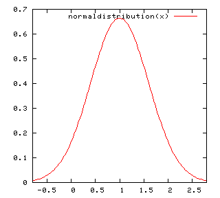
Normal Distribution. mean=1, std=0.6 
$$
$$
normaldistribution(x)=exp(-(x-1)**2/(2*(0.6)**2))/(sqrt(2*pi)*0.6)
rx=3*0.6
plot [1-rx:1+rx] normaldistribution(x)
test 

테스트 중입니다.
test2 

--
Karnes 2005-12-29 00:14:44
latex processor 코드 테스트

테스트 중입니다. 위의 것은 이상없음
![\begin{itemize}
\item[가나다] 우리나라
\item[라마바] 대한민국
\end{itemize}](/wiki/_cache/latex/79/79784f3766d69bafdecb3ed782193e37.png "\begin{itemize}
\item[가나다] 우리나라
\item[라마바] 대한민국
\end{itemize}")
이것은 어떨는지요?
다시 테스트 중입니다. 이곳은 마음껏 테스트를 위한 곳입니다.


![[http]](/wiki/imgs/http.png)


.png "B)") 123tyt굣ㅛㅅㅅㄱㄳ견ㅇ탸ㅏfdsarㅏgbvfdwgregregqㅓㅊ허ㅠㅊv+987{il}
32
123tyt굣ㅛㅅㅅㄱㄳ견ㅇ탸ㅏfdsarㅏgbvfdwgregregqㅓㅊ허ㅠㅊv+987{il}
32
)*u
for i=-2.4 step 0.1 until 2.5: --(i,sind(i*t))*u endfor;
px=(-4u,0)--(4u,0); py=(0,-2u)--(0,2u);
fill buildcycle(ps, px, py shifted (2u,0)) withcolor blue;
fill buildcycle(ps, px, py shifted (-2u,0)) withcolor red;
drawarrow px; % X-axis
drawarrow py; % Y-axis
draw ps; % Sine curve")

.png ":)")

 에 대하여 역원
  가 존재한다. :
 이 집합의 어떤 원소와 같다. :
\times{}c=a\times{}(b\times{}c) $$")
 .
.

\quad (i,j=1,2,\ldots, N) $$")
![$$ \sum'\sqrt[n]{10} $$](/wiki/_cache/latex/f2/f2a963e1a28ac699d24c691ed77418f3.png "$$ \sum'\sqrt[n]{10} $$")
;y=x rotated -120;z=u*(0,1);
path s,h,sh;s=origin--x--x+y--y--cycle;h=origin--z;sh=x--x+y--x+y+z--x+z--cycle;
draw s;
draw s shifted z;
draw h;draw h shifted x;draw h shifted x+y;draw h shifted y;
fill sh withcolor .3white;")


![\newlength\mylen
\settowidth{\mylen}{$ 2k $}
\[
\underbrace{(k+1) \le 2k}
\hskip-\mylen\overbrace{\hphantom{2k}<2\cdot 2^k} <2^{k+1}
\]](/wiki/_cache/latex/5d/5d3df468cb483bf21b02d2fae64171f0.png "\newlength\mylen
\settowidth{\mylen}{$ 2k $}
\[
\underbrace{(k+1) \le 2k}
\hskip-\mylen\overbrace{\hphantom{2k}<2\cdot 2^k} <2^{k+1}
\]")
![\newlength\mylen
\settowidth{\mylen}{$(k+1) \le 2k$}
\[
\underbrace{(k+1) \le 2k}
\hskip-\mylen\hphantom{(k+1) \le}\overbrace{\hphantom{2k}<2\cdot 2^k} <2^{k+1}
\]](/wiki/_cache/latex/ca/ca273ab9601364cbca2c8b8f1aee4374.png "\newlength\mylen
\settowidth{\mylen}{$(k+1) \le 2k$}
\[
\underbrace{(k+1) \le 2k}
\hskip-\mylen\hphantom{(k+1) \le}\overbrace{\hphantom{2k}<2\cdot 2^k} <2^{k+1}
\]")
